shot
shot
shot
Sandia National Laboratories is a multimission laboratory managed and operated by National Technology & Engineering Solutions of Sandia, LLC, a wholly owned subsidiary of Honeywell International Inc., for the U.S. Department of Energy’s National Nuclear Security Administration under contract DE-NA0003525.
There seems to be a lot of confusion and ambiguity online about what iptables masquerading does. This is frequently encountered when you forward ports in iptables,
# port forward 22222 to 22 on 192.168.2.3
sudo iptables -t nat -A PREROUTING -i eth0 -p tcp --dport 22222 -j DNAT --to-destination 192.168.2.3:22
or force some traffic to use particular interfaces,
sudo iptables -I FORWARD -i br1 -o interface1 -j ACCEPT
iptables -I FORWARD -i br1 -o interface2 -j DROP
You frequently find that you have to follow such iptables rules up with
sudo iptables -t nat -A POSTROUTING -o interface1 -j MASQUERADE
But why?
Perhaps the easiest way to see what masquerading does is to consider the first example, where we consider the case that 192.168.1.1 is port-forwarding 22222 to port 22 at 192.168.2.3 and 192.168.2.1/24 are assigned to bridge 'br1':
# port forward 22222 to 22 on 192.168.2.3
sudo iptables -t nat -A PREROUTING -i eth0 -p tcp --dport 22222 -j DNAT --to-destination 192.168.2.3:22
sudo iptables -t nat -A POSTROUTING -o br1 -j MASQUERADE
We can actually replace the second (masquerading) rule with
sudo iptables -t nat -A POSTROUTING -o br1 -p tcp --dport 22 -d 192.168.2.3 -j SNAT --to-source 192.168.1.1
This changes the source IP of the forwarded packets to 192.168.1.1 so that the client at port 22 will know that it should reply with a source NAT address of 192.168.1.1; it will "masquerade" or pretend to have IP address 192.168.1.1 when replying to this stream so that subsequent remote replies to its messages will be sent to 192.168.1.1, where they will be port-forwarded again.
If you know that you are "masquerading" everything on a certain interface, you can concisely indicate this with the "-j MASQUERADE" and save yourself the hassle of changing the POSTROUTING rules of every port etc. you're forwarding.
A recent paper by Heimendahl et al. proves, given some assumptions that are likely satisfied in the large qubit limit, that the stabilizer extent is not generally a multiplicative measure. The stabilizer extent of a state is its minimum L1-norm with respect to the stabilizer state basis. It is a commonly used primitive in classical algorithms for sampling quantum amplitudes, i.e. simulating a quantum computer, to additive error, where the state to be approximated is a tensored product of some magic state. In the case that this magic state is a one-, two-, or three-qubit state, the stabilizer extent has been proven to be multiplicative. However, this paper proves that in the general case this ceases to be true.
A sub-multiplicative stabilizer extent implies that a smaller L1-decomposition of the tensored magic state is always possible at some large enough number of qubits. In the magic state formalism, adding more qubits corresponds to incorporating more quantum universal gates in your circuit. These classical algorithms work by sampling over these L1-decompositions so a smaller decomposition necessarily runs faster. Sub-multiplicativity thus means that there is always a more efficient classical algorithm for a large enough number of qubits than that obtained by breaking up these qubits into smaller groups and naively tensoring their L1-decompositions. Finding an optimal L1-decomposition is not a trivial task, so this can be interpreted to mean that if you work hard enough, you can always come up with a faster classical algorithm to sample quantum circuits, at least in this stabilizer extent paradigm.
The method Heimendahl et al. use to complete their proof is quite interesting. Instead of relying specifically on the properties of the stabilizer states, they define five properties of a general dictionary that are not sufficient to define the stabilizer states. Perhaps the two most pertinent properties are that this dictionary of states is subexponential in size and contains the maximally mixed state. The former allows them to make a concentration-of-measure argument to bound the maximal inner product squared between a Haar-random state and any member of the dictionary. The latter allows them to show, in the dual formulation of the L1-minimization, that there always exists a witness vector that has an inner product squared greater than one with the Haar-random state when it is tensored with itself. This prevents the stabilizer extent of this Haar-random state from being multiplicative. This last point is explained well in the paper and I would encourage anyone interested to read it for more details.
SAND No.: SAND2020-10140 W
Sandia National Laboratories is a multimission laboratory managed and operated by National Technology & Engineering Solutions of Sandia, LLC, a wholly owned subsidiary of Honeywell International Inc., for the U.S. Department of Energy’s National Nuclear Security Administration under contract DE-NA0003525.
A recent draft on the arXiv, Experimental demonstration of quantum advantage for NP verification by Centrone et al., presents a claimed demonstration of computational quantum advantage over classical computation using simple linear optics. The premise that they leverage is that NP-complete problems are difficult to find solutions to but easy to verify. However, quantum computers only need a square root of the same amount of information that a classical computer needs to verify a solution. Heuristically, a classical computer would need to “fill in” the remaining square root of information and that would require an exponential cost. This comes with a bunch of caveats, not least of which is that a classical algorithm needs different information, i.e. I was careful to talk about “amount” of information, not its content.
The authors experimentally present a simple quantum computer consisting of linear optics that they claim demonstrates this speed-up and that gets around the large amount of equipment traditionally needed to implement such a quantum phenomenon. They accomplish this by developing a different quantum verification test for the task that is more practical. As a result, they are able to get away with just using coherent states of light and leverage the Sampling Matching problem implemented by an earlier group. The authors specifically focus on the 2-out-of-4 SAT problem where a quantum verifier requires linear time to verify a quantum proof, while a classical verifier would need an exponential amount of time with the same amount of information, given the well-accepted assumption that finding a solution to NP-complete problems takes exponential time.
The authors experimentally present a simple quantum computer consisting of linear optics that they claim demonstrates this speed-up and that gets around the large amount of equipment traditionally needed to implement such a quantum phenomenon. They accomplish this by developing a different quantum verification test for the task that is more practical. As a result, they are able to get away with just using coherent states of light and leverage the Sampling Matching problem implemented by an earlier group. The authors specifically focus on the 2-out-of-4 SAT problem where a quantum verifier requires linear time to verify a quantum proof, while a classical verifier would need an exponential amount of time with the same amount of information, given the well-accepted assumption that finding a solution to NP-complete problems takes exponential time.
SAND No.: SAND2020-10139 W
Sandia National Laboratories is a multimission laboratory managed and operated by National Technology & Engineering Solutions of Sandia, LLC, a wholly owned subsidiary of Honeywell International Inc., for the U.S. Department of Energy’s National Nuclear Security Administration under contract DE-NA0003525.
I have a home theater PC connected to an audio-video-receiver (AVR) and a TV. This is just a normal PC. So, after turning my TV and AVR on with their remotes, I would have to walk over to the PC and turn it on by pressing its power button. This was a bit annoying. Since I have to walk over to the TV and AVR anyway to turn on the PC, I might as well turn everything on and not benefit from the convenience of remote control.
So I decided to build an IR receiver and remote (transmitter) to remedy this, admittedly mild, inconvenience. My set-up requires that my new remote signal not trigger the other receivers in the TV and AVR. I didn't want to deal with digital circuit logic (and coding up a PAL, FPGA, or Arduino etc.) and preferred an analog circuit. At first I thought this would be difficult to do with analog components. However, after examining how IR remotes generally work and how different signals are encoded, I discovered this is a lot more straightforward.
Almost all IR remotes transmit at a "carrier" frequency of 30-40 kHz and then modulate the amplitude on/off to encode messages. We're going to use this to our advantage in producing a simple analog circuit that transmits a signal that none of the other receivers will decode to a meaningful message; we're just going to transmit the carrier frequency, i.e. a null signal according to all the other receivers.
This strategy will also allow us to build a particularly simple receiver. We can simply put the received signal through a low-pass filter that will filter out any signals higher than our carrier frequency. A low-pass is an integrator. Any IR signal that will be sending a message to the other devices will be modulating the amplitude and so be sending fewer "on" pulses at the carrier frequency in a given interval of time. Hence, the signal will integrate to a smaller area in that time interval. If we "bleed" the area at the correct rate (by adding a grounded resistor to our RC integrator) then we can ensure that only a "clean" unmodulated carrier signal produces enough area to surpass a comparator's threshold, which can then send a logical "ON" level to our computer's power supply.
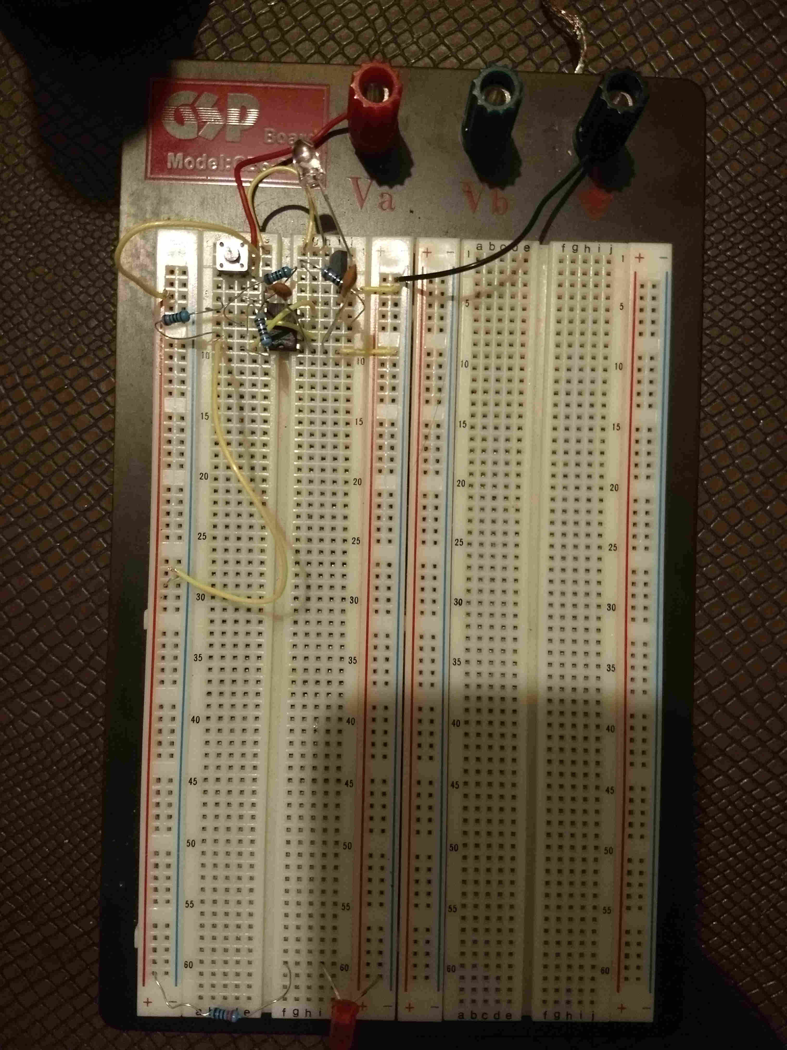
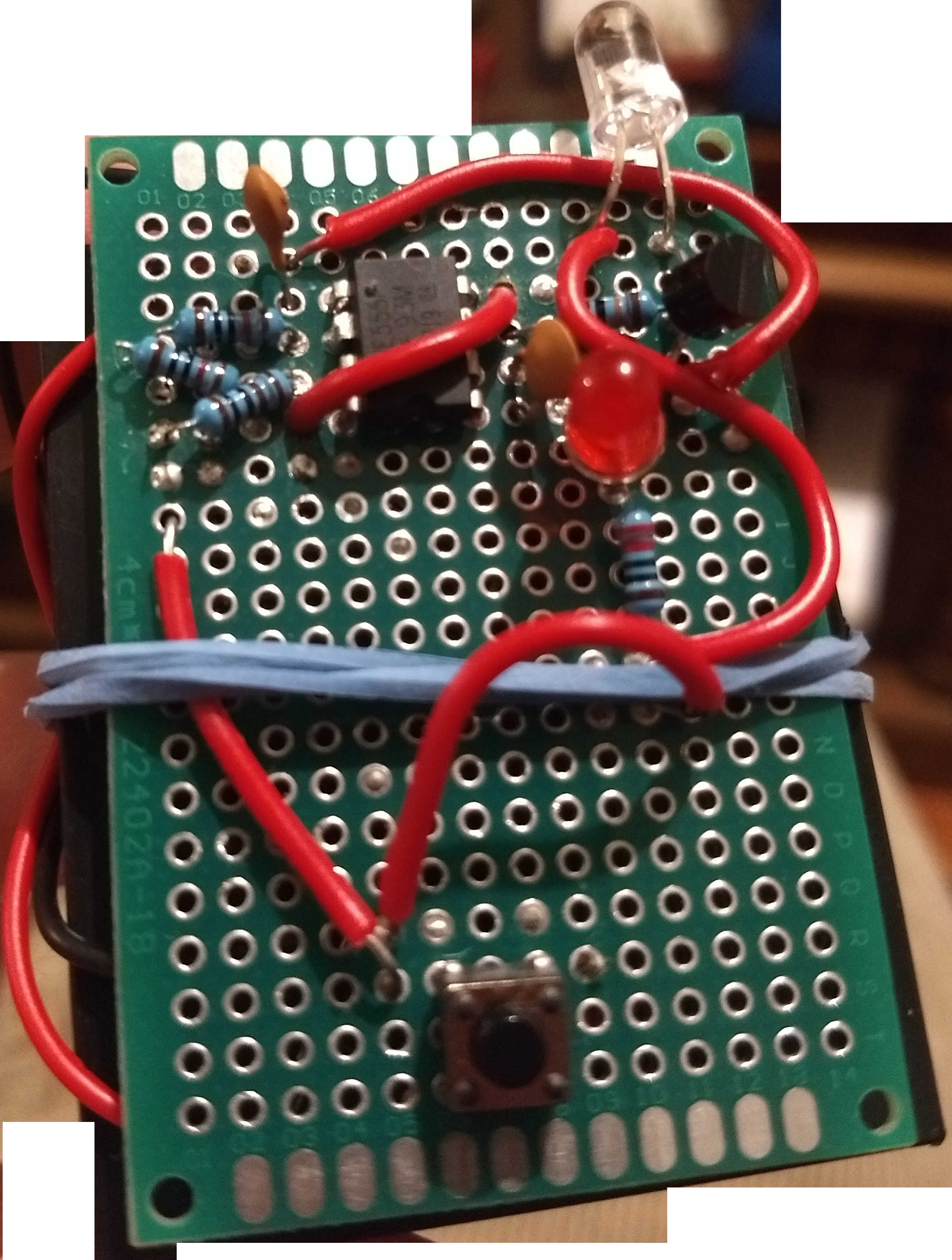
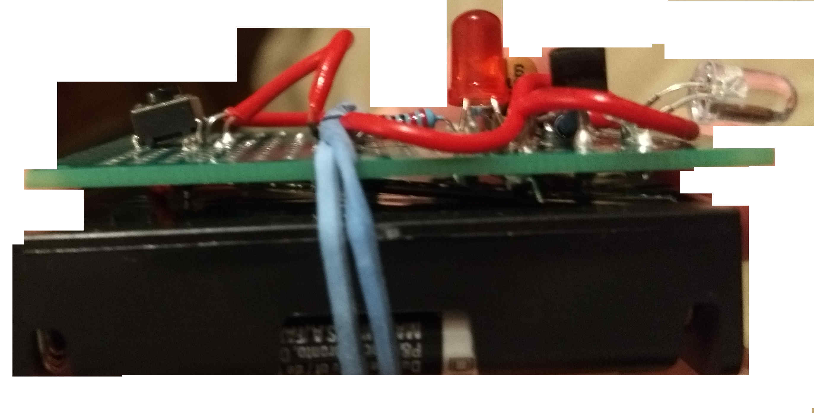
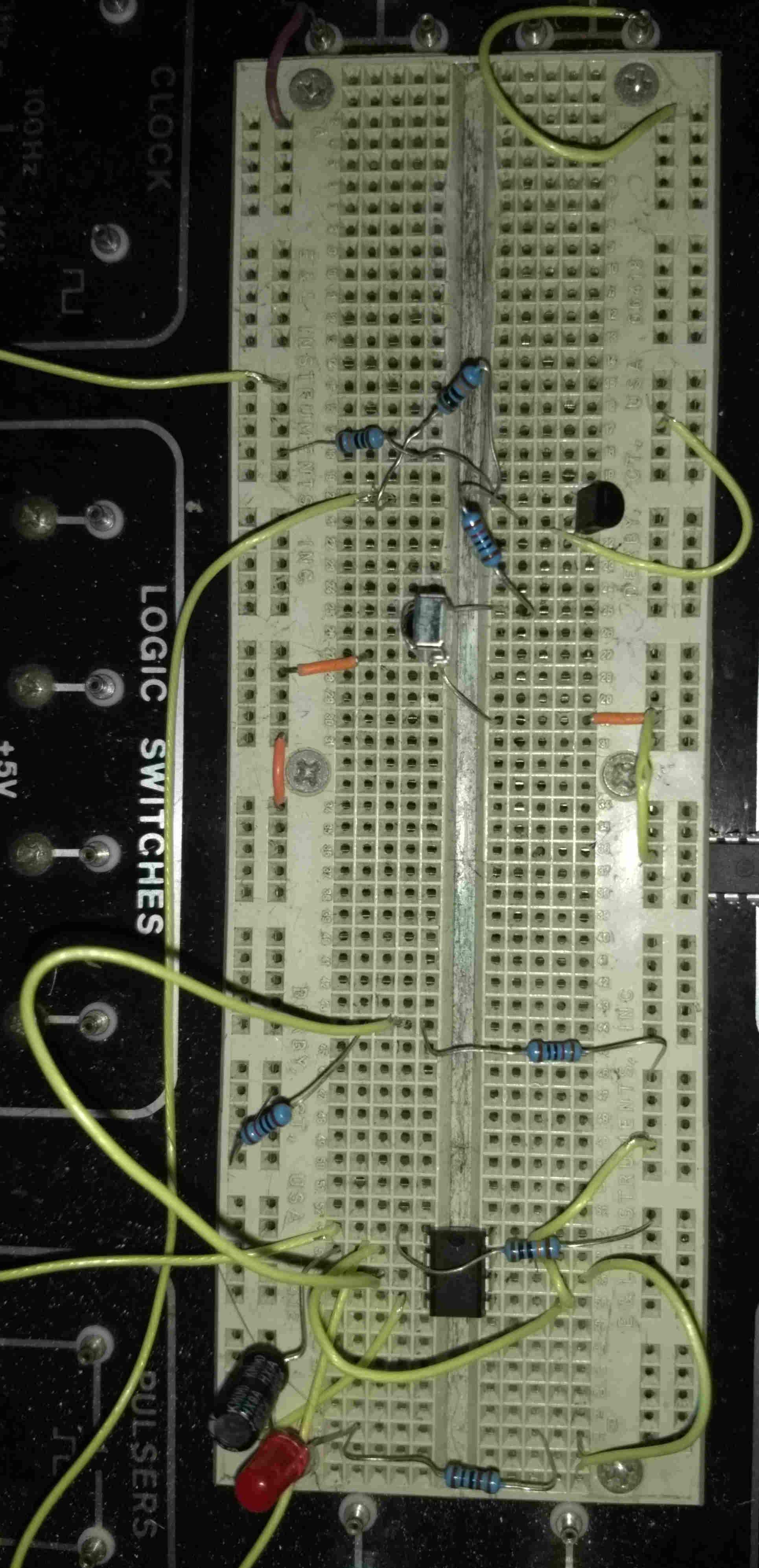
Take a look at the overall IR transmitter schematic [PDF], IR receiver schematic [PDF], and pictures of both:
| |
|
|
|---|---|---|
| Breadboard shot |
Overhead shot |
Profile shot |
 |
 |
 |
 |
 |
|---|---|---|---|---|
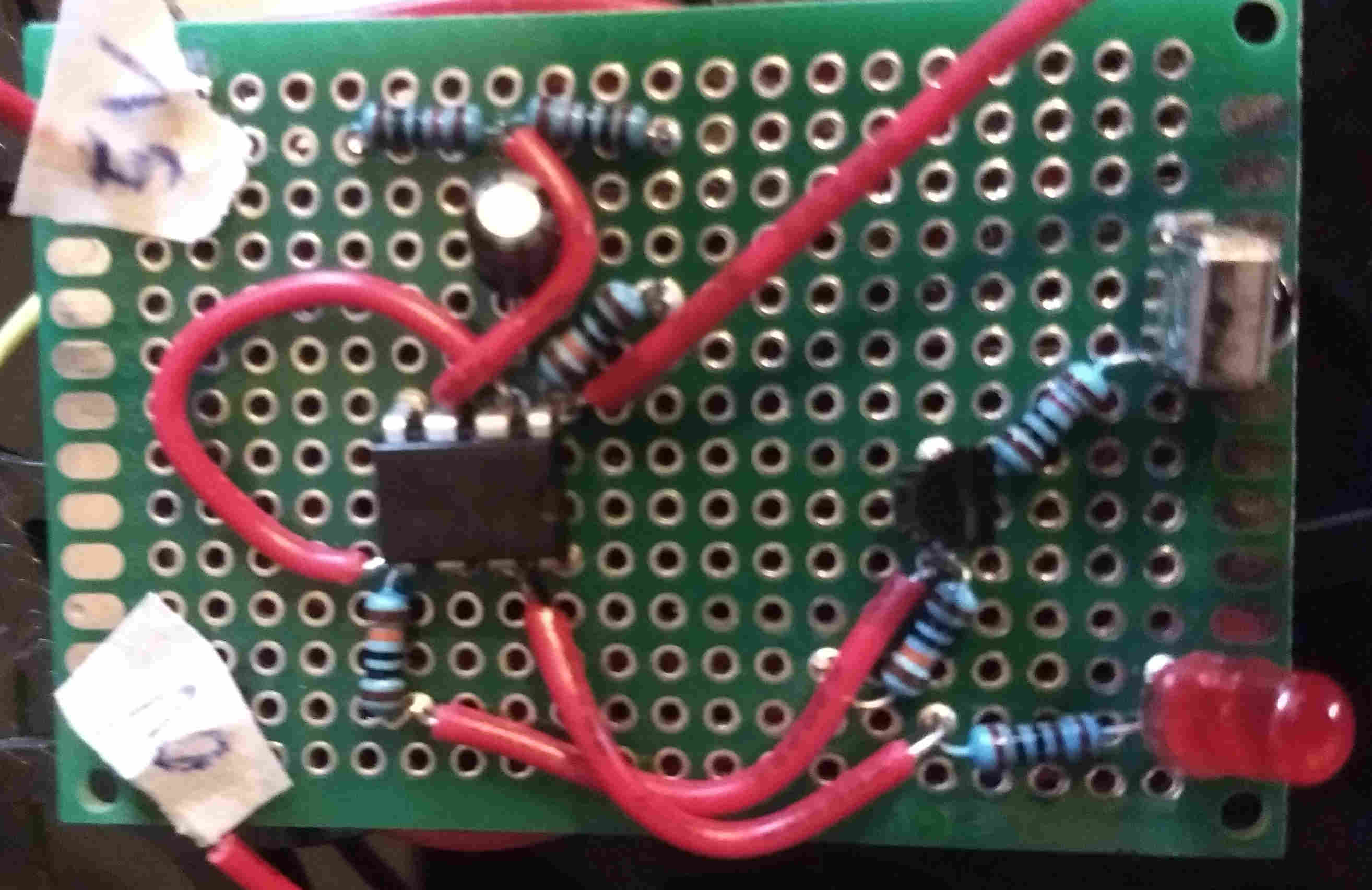
| Breadboard | Top shot |
Bottom shot |
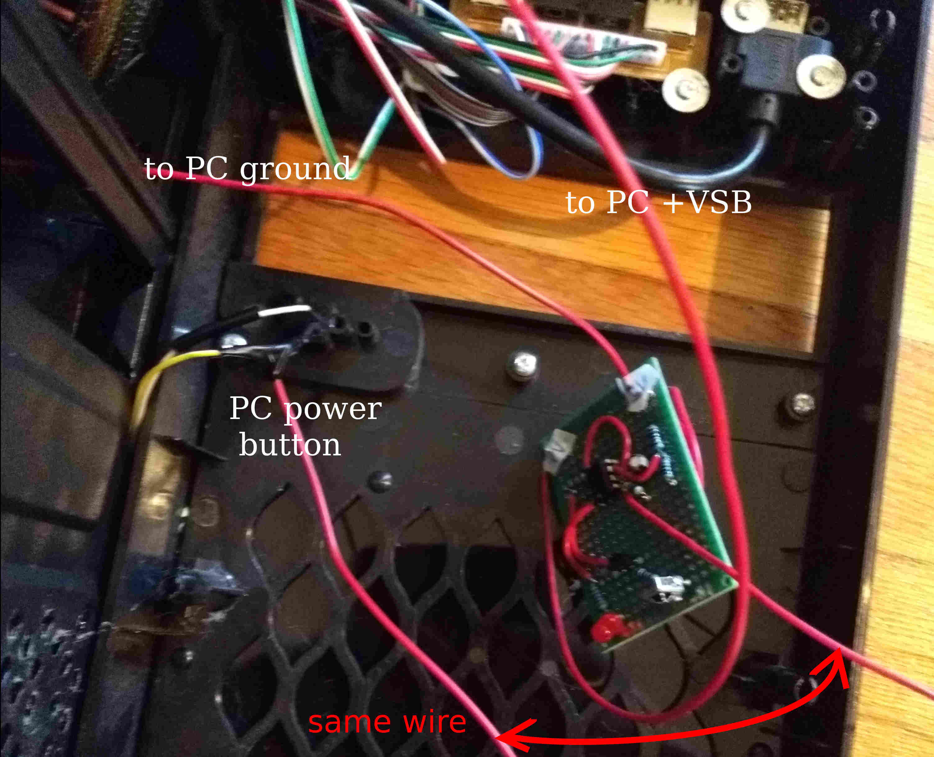
PC wire connections |
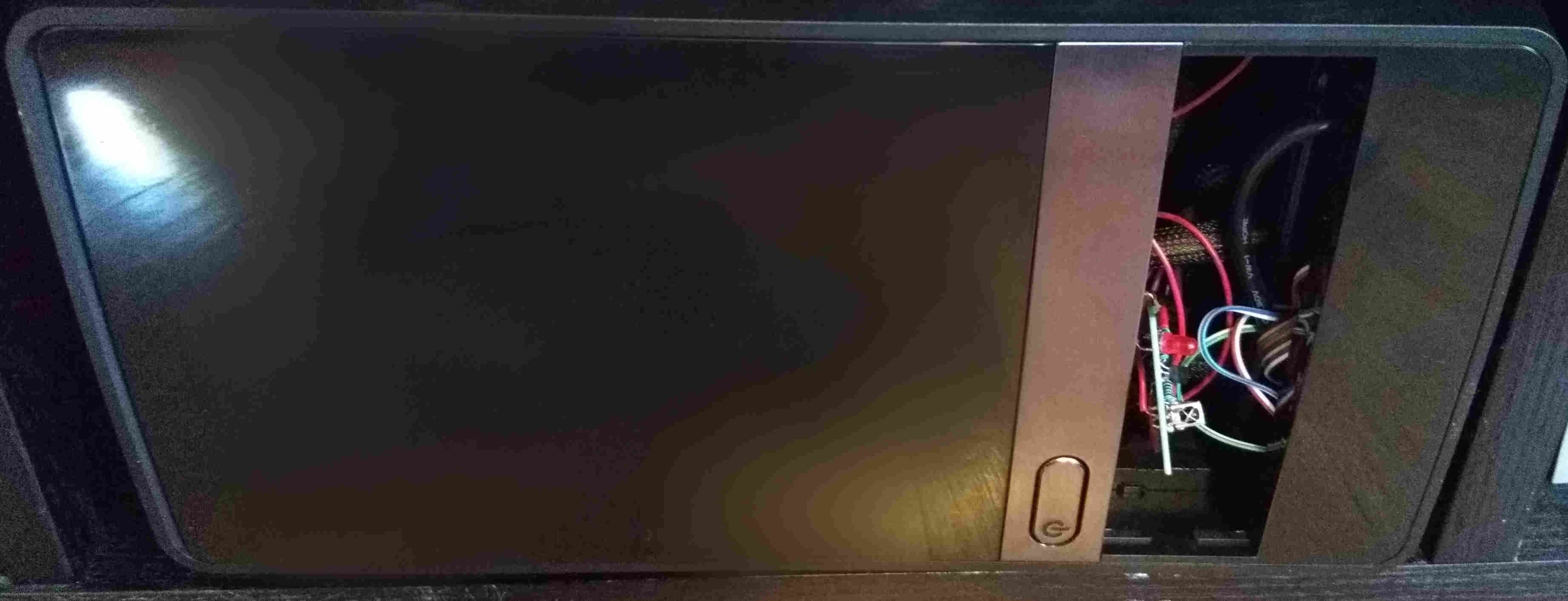
Fully installed |
So how does this work?
Let's start with the IR transmitter. The 555 timer is connected to be in an astable mode duty cycle, which has the following frequency (see the schematic PDFs for , and C):
You can read about this formula's derivation in many other excellent sources online so I won't get into that. The output of the 555 is passed to a 3904 NPN transister that acts as a switch to run sufficient current through the IR LED. It flashed on and off at the carrier frequency of 35 kHz.
I also added a red IR to the circuit that lights up when you power circuit so you know something is happening when you press the remote's button.
The IR receiver uses the TL1838 sensor integrated chip to pick up the IR signal. It actually likes a carrier signal of 38 KHz, but our 35 KHz signal is close enough. This needs 5 V at pin 3 and ground at pin 1. It outputs the amplitude it senses at pin 2. Note that it outputs the signal without the carrier frequency. This resultant signal still consists of square (ON/OFF) waves, and so I pass pin 2's output to drive a PNP 3906 transister switch--a follower and will pull more current for the rest of the circuit.
The signal on the other side of transistor is sent through a RC low-pass filter with an 1/2πRC constant of 160 Hz. It attenuates the amplitude of 160 Hz sinusoidal signals by about 70%. Higher frequency sinusoidal signals are attenuated more. Now, our signals consist of square waves, which have high frequency components at their abrupt/discontinuous slope changes. The bare carrier frequency signal will be output by the TL1838 as a steady DC high and so will be devoid of such high frequencies. So you can think of the modulated carrier signal as possessing more higher frequency sinusoidal components because it changes slope more often. As a result, modulated carrier signals will be filtered more. This integrated area is continually "bled" by the 100 kΩ resistor to ground. If the TL1838 sensor receives sufficiently pure 35 KHz carrier signal, then it is able to drive the area produced by the RC integrator high enough to combat this bleed. I chose the values of the RC constant and the bleed resister by trial and error.
Op amp A serves as a comparator. When enough signal passes through the high-pass filter such that the filter has integrated the area and raised the voltage to above 2.5 V (as set by that voltage divider with the two 10 kΩ resistors), then the inverting op amp ratchets to low (0 V at pin 1). We pass this signal to our power button wire to turn the computer on (or off).
Op amp B acts as a simple follower that sees how much signal passes the filter and lights up the red LED according to the amplitude that has passed through. This LED serves to give us some indication how much signal is passing through when we're flashing our IR remote at the receiver. It lights up a bit when I use my other remotes but only fully lights up when I send it a bare carrier signal.
You want the receiver to share the same +5 V and ground lines as the computer's motherboard. It turns out that on modern ATX power standards, the (usually red) +5 V line is not on when the computer is off. However, the (usually purple) +5 VSB (the standby voltage) is always on, so that's what you want to connect to. It's usually most easily accessible on the ATX 24 pin connector you plug from your power supply unit (PSU) to the motherboard. The PC's ground can be found in this same connector at multiple pins corresponding to its black wires.
And that's it. As you can see, it's a pretty simple set of circuits. I think the remote looks a bit gnarly, but it's the process of making it that counts. You can get away with using some cell phones as "IR blasters" if you don't want to build that part. The receiver also has a bit of a scary look in the PC (see the last picture). I might cover it with a panel that has two small holes for the red LED and the TL1838 sensor to give it a more "professional" look. I've been using it for over half a year now and enjoy this little device's compact simplicity.
Sandia National Laboratories is a multimission laboratory managed and operated by National Technology & Engineering Solutions of Sandia, LLC, a wholly owned subsidiary of Honeywell International Inc., for the U.S. Department of Energy’s National Nuclear Security Administration under contract DE-NA0003525.
I'd like to highlight a paper recently posted on the arxiv (arxiv:1902.04764 v2) by Matthias Englbrecht and Barbara Kraus at the University of Innsbruck, in Austria.
Stabilizer states are an important subject in fault-tolerance and understanding the power and cost of universal quantum computation, and this paper seems to advance their characterization for qubits in terms of their local symmetries and provides an algorithm for finding them.
The main foundational tool that Englbrech and Kraus use during their characterization is that it is sufficient to study all stabilizer states by restricting to graph states, since any stabilizer state can be related to a graph state by a local Clifford transformation (which are trivial to additionally characterize). So, there exists equivalence class of stabilizer states corresponding to the graph states. To be more precise, given an abelian subgroup of the n-qubit Pauli group not including -I a stabilizer state is the unique eigenstate for all elements of this subgroup with eigenvalue +1. It can be shown that this abelian subgroup can be generated by n Pauli operators.
Given a undirected graph G(E,V) with edges E and vertices V, the corresponding graph state is given by
where denotes the controlled phase gate on qubits i and j. This is a stabilizer state with generators
So this defines the equivalence class of stabilizer states that are equivalent up to local Clifford transformations.
They then proceed to show that there are two different types of graph states:
The symmetry group of the first type of graph state has to be a subgroup of the local Clifford group and is therefore discrete and finite.
Graph states of the second type have a continuous unitary symmetry iff the corresponding graph has a leaf up to local complementation.
I would be interested to see how this plays out for odd-dimensional qudit stabilizer states where the analysis might be simpler. I also wonder how non-local symmetries characterize the stabilizer states. Nevertheless, this gives a nice handle on how these stabilizer states "look" in terms of their (local) symmetries, which is especially important from the perspective of studying their entanglement properties.
SAND No.: SAND2020-1612 W
Sandia National Laboratories is a multimission laboratory managed and operated by National Technology & Engineering Solutions of Sandia, LLC, a wholly owned subsidiary of Honeywell International Inc., for the U.S. Department of Energy’s National Nuclear Security Administration under contract DE-NA0003525.
On page 12 of PRX 6,021043 (2016), Bravyi et al. discuss an Monte Carlo algorithm they use to try and find the smallest set of stabilizer states that spans a given state called a "magic" state. They write:
"Since our target state has real amplitudes in the computational basis, one can easily show that the optimal decomposition Eq.(B1) can be chosen such that all stabilizer states have real amplitudes as well (the real part of a stabilizer state is either zero or proportional to a stabilizer state). Accordingly, we restrict the random walk to the subset corresponding to real stabilizer states. Clearly, a move maps real states to real states if P contains even number of Y’s. The move is accepted only if this condition is satisfied."
Despite their claim that this is clear, I thought this could use some clarification. In particular, I want to clear up what I think they mean by "real part of a stabilizer state".
I believe that the authors are just expressing the fact that, in terms of the computational basis states, you can write qubit stabilizer states in terms of a linear combination of two stabilizer states, where the first only has real coefficients and the second has purely imaginary coefficients. So for instance:
a stabilizer state with stabilizer generators YI & IY can be written as: ... and
a stabilizer state with stabilizer generators XI & IY can be written as: , etc.
Any stabilizer state can be expressed as:
,
where has stabilizers that are just in terms of Xs and Zs.
Therefore, in order to maintain that the stabilizers of are just composed of Xs and Zs, you can only use Pauli projectors that have pairs of Ys. In other words, to project from one state that is has to another with , you must have pairs of Ys.
Maybe this clarification proves useful for some future reader.
SAND No.: SAND2019-11569 W
Sandia National Laboratories is a multimission laboratory managed and operated by National Technology & Engineering Solutions of Sandia, LLC, a wholly owned subsidiary of Honeywell International Inc., for the U.S. Department of Energy’s National Nuclear Security Administration under contract DE-NA0003525.
Nathan Wiebe gave a talk at a conference on "Quantum Machine Learning" at Purdue on work that he's done on a class of neural networks of Boltzmann machines. These are characterized by each neural network mode having a probability function of . Typically is chosen to be the Ising Hamiltonian and you want to change its coefficients such that the energy is minimized for what you're trying to identify:
and
where
is the KL divergence,
Quantizing this to a quantum Ising model is thought to have no classical analog when a transverse term is added (the transverse Ising model).
Unlike previous studies that have followed the classical route and trained by using the KL divergence, Nathan measured training by using the quantum relative entropy between the two quantum distributions. Relative entropy is defined as
Though this solves some issues related to using the KL divergence, it becomes very difficult when you have "hidden" layers in your neural network. Hidden layers are units in your neural network that are distinguished from "visible" layers by not being related to physical quantities. They generate correlations between the visible units. This is problematic in the quantum realm since this means that they can produce entanglement, which when traced away to just look at the visible layers, will necessarily lead to the remaining states approaching maximally mixed states. Since the eigenbasis index is what is used in these quantum Boltzmann devices as the classifier index (e.g. if you're training your neural network to pick out cats from a set of picutres, the second eigenstate might correspond to a picture of a dog and so you would want it to have a larger eigenvalue than those held by eigenstates that correspond to cats), a maximally mixed state is useless for classification.
Nathan largely addresses this problem by assuming that the hidden layer Hamiltonians commute though he also has a more general method (that is correspondingly much more expensive). There are also mathematical issues with using the relative entropy and difficulties with taking its gradient. To address this he used Jensen's inequality to get a simpler variational upper bound on the objective function and used this in the gradient calculations.
On the subject of the power of quantum machine learning compared to classical machine learning, Nathan noted that with classical machine learning, you can only change the energy surface while with quantum machine learning you can also change the eigenbasis. This, along with other reasons, form the crux of his argument for why quantum machine learning has the potential to solve more problems than classical machine learning: quantum Boltzmann machines are more expressive than classical Boltzmann machines unless BQB=BPP. This seems to largely follow the argument he published some time ago (arXiv:1412.3489).
This is a pretty interesting approach to machine learning that introduces a novel approach to training when using quantum Boltzmann machines.
Sandia National Laboratories is a multimission laboratory managed and operated by National Technology & Engineering Solutions of Sandia, LLC, a wholly owned subsidiary of Honeywell International Inc., for the U.S. Department of Energy’s National Nuclear Security Administration under contract DE-NA0003525.
There is an interesting paper on the arxiv (arxiv:1902.04764 v2) by Tomoyuki Morimae and Suguru Tamaki at Kyoto University.
They demonstrate that strong simulation of the Clifford+T-gateset must scale as up to an exponentially small additive error by relying on the Exponential-Time Hypothesis, instead of the traditional appeal to the non-collapse of the polynomial time hierarchy. It also shows that the corresponding weak simulation sampling problem within a constant multiplicative error must scale as . They then suggest that this implies that strong simulation algorithms that calculate up to some constant multiplicative error cannot be subexponential (and so, for instance is not possible).
This is interesting because, in general, weak simulation is not necessarily less costly than strong simulation. So it is surprising that they are using a lower bound on weak simulation results to lower bound a strong simulation result. However, this is probably fine since weak simulation of the Clifford+T gateset is thought to be easier than its strong simulation (certainly all classical algorithms have so far shown this to be the case).
We are in the age of intermediate-size quantum computers without error-correction---so called noisy intermediate scale quantum (NISQ) computers---and we are reaching the limit of quantum circuits that can be validated by classical computers [1]. All the major industrial players in classical computing---IBM, Microsoft, Google, Intel etc.---and many start-ups are involved in trying to build such a NISQ computer. They have publicly expressed the need for better and newer algorithms for classical simulation of quantum circuits to validate and verify whether their efforts truly result in a "quantum" machine. Moreover, it is important to also establish whether their eventual machines are offering quantum "advantage" or "supremacy" over their classical counterparts---i.e. can they perform their task faster than our current computers.
Moreover, classical algorithms are necessary for breaking up quantum algorithms in the near-term due to their small size. It will be very helpful to find as many parts of a quantum algorithm that are classically efficiently simulable and so can be run in parallel on a classical computer, producing a hybrid classical-quantum computer that still demonstrates quantum "advantage". This is important for algorithms prevalent in chemistry, such as the variational quantum eigensolver (VQE) [2-4], for calculating properties of condensed matter [5], and many others [6,7].
One of the most compelling reasons for using a semiclassical approach is that it directly relates quantum phenomena to classical mechanics and provides a formal and exact relationship between the two, governed by ħ. Calculating or computing quantum evolution by including only low-order ħ terms is usually more computationally tractable than full quantum evolution as it is representable by a classical probability theory with integrable dynamics.
Continuous systems are characterized by infinite-dimensional Hilbert spaces (i.e. a particle's position can take on any value on the real line) while discrete systems are characterized by finite-dimensional Hilbert spaces (i.e. a particle's position can only take on discrete values, like the natural numbers up to some bound). Quantum computers are typically defined on the latter and define their fundamental unit of information to be a qubit---a quantum state that can only take two discrete values.
Whereas the application of a semiclassical path integral approach to continuous (infinite-dimensional) systems is long-established, its use for discrete systems is in a far more nascent stage. The notion of classicality in quantum information and related topics, including contextuality, entanglement and quantum "coherence", has until now resided within the language of complexity classes developed in computer science and entropic (or "thermodynamic") definitions [30-33]. Similarly, the practical side of the simulation of quantum algorithms has generally been accomplished by quantum Monte Carlo methods or tensor network approaches. I think it is time for the discrete version of methods that have been developed and found to be useful in continuous Hilbert spaces, such as WKB methods and their higher order corrections [34] and level-spacing trace formulas [35], to be developed and introduced. There has even been a lot of work done in the continuous setting on developing "minimally quantum" corrections to classically efficient propagators (so-called Feynman-Vernon influence functionals) that serve as incredibly promising candidates, when discretized, as quantum algorithm candidates for NISQ computers to handle in a hybrid classical-quantum manner. I have taken the first few steps in the direction of bringing such semiclassical methods to bear in the discrete world with my work on the classical simulation of quantum circuits composed of Clifford+T-gates [36], but there is far more to do.
[1] J. Preskill. Quantum Computing in the NISQ era and beyond. ArXiv e-prints, January 2018.
[2] Alberto Peruzzo, Jarrod McClean, Peter Shadbolt, Man-Hong Yung, Xiao-Qi Zhou, Peter J Love, Alán Aspuru-Guzik, and Jeremy L Obrien. A variational eigenvalue solver on a photonic quantum processor. Nature communications, 5:4213, 2014.
[3] Jarrod R McClean, Jonathan Romero, Ryan Babbush, and Alán Aspuru-Guzik. The theory of variational hybrid quantum-classical algorithms. New Journal of Physics, 18(2):023023, 2016.
[4] Dave Wecker, Matthew B Hastings, and Matthias Troyer. Progress towards practical quantum variational algorithms. Physical Review A, 92(4):042303, 2015.
[5] Bela Bauer, Dave Wecker, Andrew J Millis, Matthew B Hastings, and Matthias Troyer. Hybrid quantum-classical approach to correlated materials. Physical Review X, 6(3):031045, 2016.
[6] Juha M Kreula, Laura Garcı́a-Álvarez, Lucas Lamata, Stephen R Clark, Enrique Solano, and Dieter Jaksch. Few-qubit quantum-classical simulation of strongly correlated lattice fermions. EPJ Quantum Technology, 3(1):11, 2016.
[7] Ryan Babbush, Nathan Wiebe, Jarrod McClean, James McClain, Hartmut Neven, and Garnet Kin Chan. Low depth quantum simulation of electronic structure. arXiv preprint arXiv:1706.00023, 2017.
[8] Andrew M Gleason. Measures on the closed subspaces of a hilbert space. Journal of mathematics and mechanics, 6(6):885–893, 1957.
[9] Simon Kochen and E.P. Specker. The problem of hidden variables in quantum mechanics. Journal of Mathematics and Mechanics, 17(0):1, 1967.
[10] Harold Ollivier and Wojciech H. Zurek. Quantum discord: A measure of the quantumness of correlations. Phys. Rev. Lett., 88:017901, Dec 2001.
[11] Mark Howard, Joel Wallman, Victor Veitch, and Joseph Emerson. Contextuality supplies the ’magic’ for quantum computation. Nature, 510(7505):351–355, 2014.
[12] C Chester, B Friedman, and F Ursell. An extension of the method of steepest descents. In Mathematical Proceedings of the Cambridge Philosophical Society, volume 53, pages 599–611. Cambridge Univ Press, 1957.
[13] MC Gutzwiller. Mc gutzwiller, j. math. phys. 12, 343 (1971). J. Math. Phys., 12:343, 1971.
[14] Kocia, Lucas, and Peter Love. "Stationary Phase Method in Discrete Wigner Functions and Classical Simulation of Quantum Circuits." arXiv preprint arXiv:1810.03622 (2018).